Table of Contents
Introduction: Quantum Computer Anatomy Begins – Why This Machine Looks Alien
A Quantum Computer is not simply a faster classical computer with upgraded parts. It operates on principles that defy everyday intuition, housed within machinery that looks more like a laboratory apparatus than any recognizable computing device. The physical form of a Quantum Computer resembles a chandelier suspended in a cylindrical chamber, its golden layers descending through stages of progressively colder temperatures until reaching conditions colder than outer space. This article opens that mysterious enclosure and reveals the anatomy of a Quantum Computer, component by component, explaining why each part must exist and how they work together to enable computation through quantum physics.
The components inside a Quantum Computer serve one unified purpose: protecting and manipulating quantum states that nature tries to destroy within microseconds. Every element, from the outer casing to the processor buried at the coldest point, exists because quantum information is extraordinarily fragile. Understanding these components means understanding why this technology cannot simply be shrunk into a laptop or smartphone. The architecture revealed here explains both the power and the limitations of quantum computing.
Quantum Computer Basic Characteristics
| Aspect | Description |
|---|---|
| Operating Temperature | 15 millikelvin, approximately 180 times colder than interstellar space |
| Physical Size | Systems range from refrigerator-sized units to room-filling installations |
| Primary Computing Element | Superconducting circuits or trapped ions acting as qubits |
| Environmental Requirement | Near-perfect vacuum and electromagnetic isolation |
| Computational Approach | Parallel exploration of solution spaces through quantum superposition |
| Error Rate Challenge | Quantum states degrade within 100 microseconds in current systems |
| Classical Interface Dependency | Requires conventional computers for control, calibration, and readout |
| Application Domain | Optimization problems, molecular simulation, and cryptographic tasks |
1. Quantum Computer Qubits: The Core Information Carriers
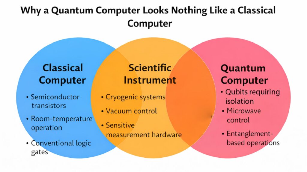
Qubits represent the fundamental computing units inside a Quantum Computer, yet they bear little resemblance to the transistors in classical machines. A qubit is a physical system that can exist in quantum superposition, meaning it occupies multiple states simultaneously until measured. In most commercial Quantum Computers today, qubits take the form of superconducting circuits fabricated on silicon chips, cooled to temperatures where electrical resistance vanishes. IBM, Google, and Rigetti use this approach. Other implementations employ trapped ions suspended in electromagnetic fields or photons manipulated through optical systems.
The physical reality of qubits determines everything else about Quantum Computer design. These are not abstract mathematical constructs but actual pieces of matter or energy configured to maintain quantum coherence. A superconducting qubit consists of a Josephson junction, a thin insulating barrier between two superconductors, coupled to microwave resonators. Ion trap qubits use individual atoms held motionless by electric fields. Each approach faces the same challenge: quantum states naturally decay through a process called decoherence, typically within 100 microseconds for superconducting qubits.
Every other component in a Quantum Computer exists to serve qubits. The refrigeration keeps them superconducting. The shielding blocks environmental interference. The control lines send precise signals. The measurement hardware reads their final states. Without maintaining qubit coherence, quantum computation becomes impossible. This fragility explains why Quantum Computers cannot operate at room temperature and why scaling them remains difficult. Current systems from IBM contain between 27 and 433 qubits, while Google’s Sycamore processor uses 53 qubits. These numbers remain modest compared to billions of transistors in classical chips because each qubit requires extensive supporting infrastructure.
The quality of qubits determines computational capability more than their quantity. Researchers measure qubit performance through coherence time, gate fidelity, and connectivity. Coherence time indicates how long quantum information persists before decaying. Gate fidelity measures the accuracy of operations performed on qubits. Connectivity describes which qubits can directly interact. Google reported coherence times exceeding 100 microseconds for their qubits in 2019. IBM has demonstrated two-qubit gate fidelities above 99 percent. These metrics improve gradually, but physics imposes hard limits on how much better qubits can become without fundamental architectural changes.
Quantum Computer Qubit Implementation Methods
| Qubit Type | Physical Basis |
|---|---|
| Superconducting Qubits | Josephson junctions in superconducting circuits operating below 20 millikelvin |
| Trapped Ion Qubits | Individual atoms suspended in electromagnetic fields using laser manipulation |
| Photonic Qubits | Single photons encoded in polarization or path states transmitted through waveguides |
| Topological Qubits | Exotic quantum states called anyons protected by topology rather than isolation |
| Neutral Atom Qubits | Atoms trapped in optical lattices created by intersecting laser beams |
| Quantum Dot Qubits | Electron spins confined in semiconductor nanostructures at millikelvin temperatures |
| Nuclear Spin Qubits | Atomic nuclei in silicon or diamond manipulated through magnetic resonance |
| Coherence Time Range | Current implementations maintain quantum states between 10 and 600 microseconds |
2. Quantum Computer Dilution Refrigerator: Extreme Cold as Infrastructure
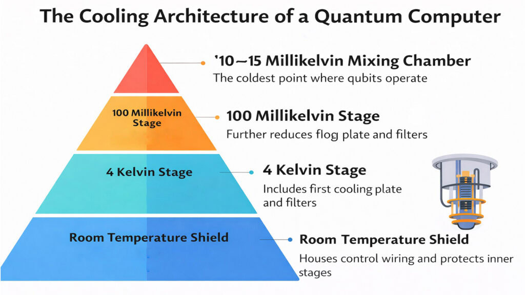
The dilution refrigerator forms the physical structure of most Quantum Computers, providing the extreme cold necessary for superconducting qubits to function. This device is not peripheral equipment but the primary architecture within which computation occurs. The refrigerator uses a mixture of helium-3 and helium-4 isotopes to reach temperatures around 15 millikelvin, roughly 180 times colder than the cosmic microwave background radiation permeating space. Without this cold, superconducting circuits would behave like normal conductors, losing their quantum properties immediately.
The refrigerator consists of multiple nested stages, each progressively colder than the last. A typical system includes four to six temperature stages descending from room temperature to the millikelvin range. The outermost stage operates around 4 Kelvin using liquid helium cooling. Inner stages employ pulse tube refrigeration and finally dilution cooling at the core. Each stage is thermally anchored but mechanically isolated to prevent vibration transmission. The quantum processor sits at the bottom stage where the temperature stabilizes below 20 millikelvin. This layered construction explains why Quantum Computers often appear as vertical cylinders with golden heat shields suspended within.
Operating a dilution refrigerator requires continuous helium circulation and careful thermal management. The cooldown process takes several days, gradually reducing temperature while preventing thermal stress on components. Once operational, the system consumes significant electrical power, typically several kilowatts, to maintain cryogenic conditions. Companies like Bluefors and Oxford Instruments manufacture these specialized refrigerators specifically for quantum computing applications. A commercial dilution refrigerator costs between 500,000 and 2 million dollars, depending on capacity and features.
The refrigerator does more than cool. It provides a stable thermal environment where quantum coherence can persist. Temperature fluctuations of even a few millikelvin can introduce errors in quantum operations. The refrigeration system actively stabilizes temperature through feedback control, monitoring thermometers at each stage and adjusting cooling power accordingly. This thermal stability proves to be as critical as reaching low temperature initially. Modern dilution refrigerators achieve temperature stability better than 0.1 millikelvin over hours of operation.
Quantum Computer Dilution Refrigerator Specifications
| Parameter | Typical Value |
|---|---|
| Base Temperature | 10 to 20 millikelvin at the mixing chamber where qubits reside |
| Cooldown Duration | 24 to 72 hours from room temperature to operating conditions |
| Cooling Power at Base | 400 microwatts at 100 millikelvin for high-performance systems |
| Number of Temperature Stages | Four to six stages cascading from 300 Kelvin to 15 millikelvin |
| Helium-3 Requirement | Several liters of helium-3, a rare isotope costing thousands per liter |
| System Height | 2 to 3 meters for typical quantum computing installations |
| Electrical Power Consumption | 5 to 25 kilowatts depending on cooling capacity and auxiliary systems |
| Vibration Isolation | Sub-micrometer displacement to prevent qubit decoherence from mechanical noise |
3. Quantum Computer Microwave Control Lines: Commanding Qubits
Microwave control lines form the communication pathway between room-temperature electronics and qubits operating at millikelvin temperatures. These carefully engineered transmission lines carry microwave pulses, typically in the 4 to 8 gigahertz range, that manipulate qubit states with nanosecond precision. Every quantum gate operation requires sending shaped microwave pulses through these lines, making them the functional nervous system of a Quantum Computer. The design and routing of control lines significantly impact system performance and scalability.
Each qubit requires dedicated control and readout lines, creating a wiring challenge that intensifies as qubit counts increase. A 50-qubit system might need 150 coaxial cables threading through the dilution refrigerator, each carefully thermalized at multiple temperature stages. These cables must conduct signals while blocking heat, a seemingly contradictory requirement addressed through specialized coaxial designs using superconducting inner conductors and stainless steel outer shields. Attenuators placed at different temperature stages reduce thermal noise traveling down the lines toward qubits.
The microwave pulses sent through control lines must achieve extraordinary precision. Quantum gate operations require controlling microwave amplitude, frequency, and phase to better than one percent accuracy over nanosecond timescales. Pulse shaping techniques smooth the onset and termination of microwave bursts to prevent unwanted qubit excitations. These shaped pulses, often called DRAG pulses after derivative removal by adiabatic gate protocols, help achieve high-fidelity quantum operations. Research from institutions like MIT and Yale has refined these pulse shaping techniques over two decades of development.
Control line engineering involves constant tradeoffs between signal quality and thermal management. Adding more attenuation reduces noise but also weakens control signals, requiring higher power amplifiers at room temperature. Using superconducting cables minimizes heat conduction but can introduce nonlinearities that distort pulses. Modern Quantum Computers employ signal multiplexing to reduce cable count, sending control pulses for multiple qubits through shared lines distinguished by frequency. This approach, demonstrated by researchers at IBM, allows addressing eight or more qubits per control line.
Quantum Computer Microwave Control System Parameters
| Component | Specification |
|---|---|
| Operating Frequency Range | 3 to 10 gigahertz depending on qubit energy level spacing |
| Pulse Duration | 10 to 100 nanoseconds for typical single-qubit gate operations |
| Cable Type | Low-loss coaxial with superconducting inner conductor and stainless steel shield |
| Attenuation Distribution | 20 to 60 decibels total attenuation distributed across temperature stages |
| Phase Stability Requirement | Sub-degree phase control to maintain gate fidelity above 99 percent |
| Room Temperature Electronics | Arbitrary waveform generators operating at gigahertz sampling rates |
| Cryogenic Components | Isolators, circulators, and directional couplers at millikelvin stages |
| Multiplexing Capacity | Up to 16 qubits addressable through frequency-multiplexed control on single line |
4. Quantum Computer Processor Chip: Where Computation Physically Occurs
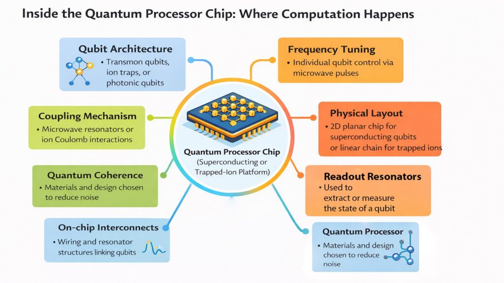
The quantum processor sits at the heart of a Quantum Computer, a silicon chip typically a few square centimeters in area, mounted at the coldest point inside the dilution refrigerator. Unlike classical processors that execute instructions sequentially, quantum processors enable computation through controlled quantum evolution. The chip contains qubits fabricated as superconducting circuits, along with coupling elements that enable qubit interaction and resonators for readout. This physical substrate determines what computations become possible.
Manufacturing quantum processor chips requires advanced fabrication techniques borrowed from the semiconductor industry but adapted for quantum requirements. Companies like IBM and Google use photolithography and thin-film deposition to pattern aluminum or niobium into superconducting circuits. The Josephson junctions that form qubits demand nanometer-scale precision. A typical junction measures about 100 by 200 nanometers, smaller than most viruses. Fabrication occurs in cleanroom facilities to prevent contamination that could introduce defects affecting qubit coherence. Intel operates a quantum chip fabrication facility in Oregon specifically for this purpose.
The processor chip layout reflects the physical constraints of quantum computation. Qubits must be close enough for controlled interactions but separated enough to prevent unwanted coupling. Most current designs arrange qubits in two-dimensional grids with nearest-neighbor connectivity. Google’s Sycamore processor uses a checkerboard pattern where each qubit connects to four neighbors. IBM’s heavy-hex lattice provides higher connectivity with qubits connecting to six neighbors, improving circuit efficiency for certain algorithms. These layout choices impact which quantum algorithms can run efficiently.
Processor chips also integrate classical circuit elements needed for control and readout. Resonators coupled to qubits enable state measurement. Capacitors provide controlled coupling between qubits for two-qubit gates. On-chip filters reduce crosstalk between adjacent qubits. Some designs incorporate flux bias lines for tuning qubit frequencies. The Quantum Computer processor remains a hybrid device, combining quantum and classical elements on the same substrate. Research groups at institutions like ETH Zurich have demonstrated processors integrating over 100 qubits with complex control circuitry.
Quantum Computer Processor Chip Architecture
| Feature | Description |
|---|---|
| Chip Size | 5 to 25 millimeters per side for current superconducting processors |
| Substrate Material | High-resistivity silicon wafers with 300 micrometer typical thickness |
| Superconducting Material | Aluminum or niobium films deposited through sputtering or evaporation |
| Junction Fabrication Method | Double-angle evaporation or Dolan bridge technique for nanoscale junctions |
| Qubit Layout Pattern | Two-dimensional arrays with nearest-neighbor or next-nearest-neighbor connectivity |
| On-Chip Resonators | Quarter-wave or half-wave resonators for qubit readout at gigahertz frequencies |
| Coupling Architecture | Tunable or fixed coupling between qubits using capacitive or inductive elements |
| Design Iteration Cycle | 6 to 18 months from design to fabricated chip including testing |
5. Quantum Computer Vacuum and Shielding Systems: Isolation from Reality
A Quantum Computer operates inside multiple layers of shielding that isolate qubits from environmental interference. This isolation serves as essential infrastructure rather than optional protection. The shielding blocks electromagnetic radiation, magnetic fields, cosmic rays, and radioactive decay from building materials. Without this isolation, quantum coherence collapses within microseconds, making computation impossible. The shielding transforms the quantum processor’s environment into something closer to deep space than Earth’s surface.
Electromagnetic shielding forms the outermost protective layer. The dilution refrigerator housing provides some shielding, but serious Quantum Computers add dedicated radio frequency shields. These shields consist of copper or aluminum enclosures with interlocking seams that prevent electromagnetic leakage. Multiple nested shields, each grounded at different points, create a Faraday cage effect that attenuates external radio signals by 100 decibels or more. Companies like ETS-Lindgren manufacture specialized RF shielding rooms for quantum computing installations.
Magnetic field shielding addresses another decoherence source. Earth’s magnetic field, though weak at about 50 microtesla, can affect superconducting qubits. Mu-metal shields, made from nickel-iron alloys with high magnetic permeability, redirect magnetic field lines around the quantum processor. Multiple layers of mu-metal, separated by air gaps, provide shielding factors exceeding 10,000. Some installations add active magnetic field cancellation using Helmholtz coils that generate opposing fields, nullifying external fluctuations. Research at Delft University of Technology has demonstrated magnetic field stability below one nanotesla using these combined approaches.
Vibration isolation prevents mechanical disturbances from reaching the quantum processor. The dilution refrigerator mounts on pneumatic isolators or active damping platforms that reduce building vibrations by factors of 100 or more above one hertz. Internal vibrations from refrigerator pumps require additional isolation through flexible couplings and careful mechanical design. Even subtle vibrations can modulate qubit frequencies or induce crosstalk between qubits. High-performance Quantum Computers achieve vibration levels below one micrometer displacement at the processor location.
Vacuum systems maintain ultra-high vacuum around the quantum processor, typically below one millionth of atmospheric pressure. This vacuum prevents air molecules from depositing on the superconducting circuits and reduces residual gas collisions that could disturb qubits. The vacuum chamber uses conflat flanges with copper gaskets to achieve leak rates below one trillionth of atmospheric pressure per second. Turbomolecular pumps and ion pumps maintain a vacuum during operation. Some systems get materials that absorb residual hydrogen and water vapor, further improving vacuum quality.
Quantum Computer Isolation System Specifications
| Isolation Type | Performance Level |
|---|---|
| Electromagnetic Shielding | 80 to 120 decibel attenuation from 10 kilohertz to 10 gigahertz |
| Magnetic Field Shielding | Residual field below 1 microtesla inside innermost magnetic shield |
| Vibration Isolation Floor | Displacement below 1 micrometer at frequencies above 1 hertz |
| Vacuum Level | 10^-9 torr or lower at quantum processor location |
| Cosmic Ray Shielding | Concrete or lead shielding reducing ionizing radiation by factor of 10 |
| Thermal Radiation Blocking | Multi-layer insulation with 40 to 60 layers reducing radiative heat load |
| Acoustic Isolation | Anechoic chamber or acoustic foam reducing airborne noise by 40 decibels |
| Electrical Grounding | Multi-point grounding scheme with impedance below 0.1 ohms at DC |
6. Quantum Computer Gates: Physical Operations on Qubits
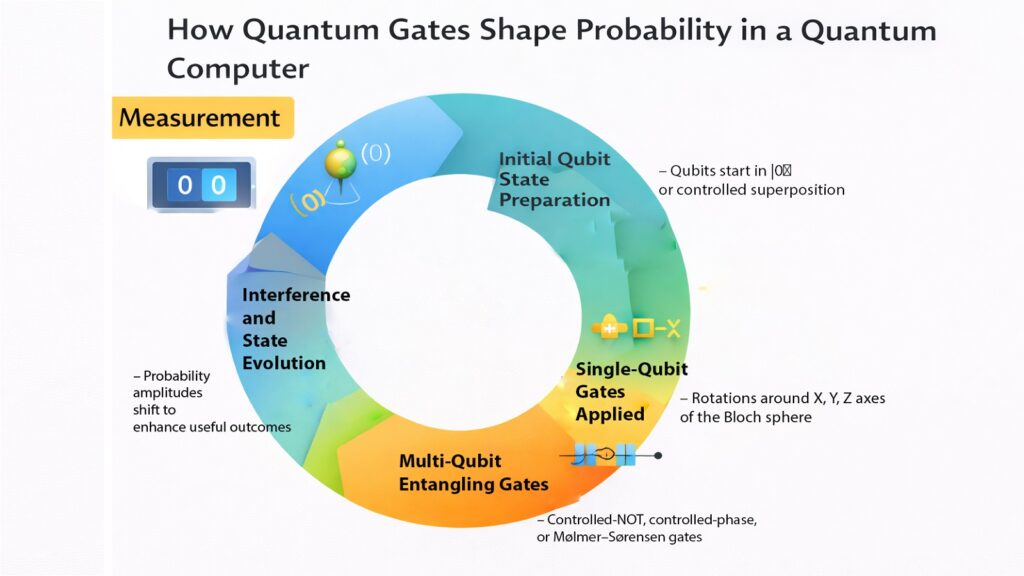
Quantum gates represent the fundamental operations that manipulate qubit states during computation. Unlike classical logic gates that switch transistors between definite on-off states, quantum gates physically rotate qubits through quantum state space. These rotations happen through carefully timed microwave pulses or laser interactions that alter quantum superposition and entanglement. Every quantum algorithm decomposes into sequences of quantum gates, making gate quality the limiting factor for computational accuracy.
Single-qubit gates rotate individual qubit states without affecting other qubits. Common single-qubit gates include the Pauli gates X, Y, and Z that flip or phase-shift quantum states, and the Hadamard gate that creates equal superposition. Physically, these operations occur through resonant microwave pulses matching the qubit’s transition frequency. A typical X gate requires a microwave pulse lasting 20 to 50 nanoseconds with amplitude calibrated to induce a complete state flip. The pulse shape matters critically, with Gaussian or hyperbolic secant profiles minimizing leakage to unwanted energy levels.
Two-qubit gates create entanglement, the quantum correlation that enables computational speedup. The CNOT gate and the controlled-phase gate represent standard two-qubit operations. Implementing these gates physically requires turning on interaction between qubits temporarily. Superconducting quantum processors achieve this through tunable coupling, where one qubit’s frequency shifts to bring it into resonance with another qubit. The interaction lasts 100 to 300 nanoseconds, enough time for quantum states to become entangled before returning qubits to their original frequencies.
Gate fidelity measures how accurately a physical gate operation matches its ideal mathematical description. Current Quantum Computers achieve single-qubit gate fidelities between 99.9 and 99.99 percent, meaning fewer than one in 1,000 operations introduce errors. Two-qubit gates prove more difficult, with typical fidelities between 99 and 99.5 percent. These error rates compound rapidly in long quantum circuits. A computation requiring 1,000 two-qubit gates would fail with near certainty at 99 percent fidelity but might succeed at 99.9 percent fidelity. Companies like IBM and Google continuously refine gate implementations to push fidelities higher.
Gate calibration requires constant attention. Qubits drift over hours and days due to environmental changes and material aging. Control systems periodically recalibrate gate parameters using automated protocols that sweep pulse amplitudes and frequencies while measuring resulting states. This calibration happens daily or even hourly for high-precision applications. Machine learning techniques increasingly optimize gate parameters, with algorithms automatically discovering pulse shapes that maximize fidelity for specific hardware.
Quantum Computer Gate Implementation Details
| Gate Type | Physical Implementation |
|---|---|
| Single-Qubit X Gate | Resonant microwave pulse at qubit frequency for half oscillation period |
| Single-Qubit Hadamard Gate | Microwave pulse combining X rotation and phase shift in single operation |
| CNOT Two-Qubit Gate | Conditional frequency shift bringing qubits into resonance for controlled interaction |
| Controlled-Z Gate | Temporary capacitive coupling inducing phase shift conditional on qubit states |
| Gate Duration Range | 10 to 50 nanoseconds for single-qubit gates, 100 to 500 nanoseconds for two-qubit gates |
| Error Sources | Decoherence during gate, pulse distortion, crosstalk, and leakage to non-computational states |
| Calibration Frequency | Daily to hourly depending on system stability and application requirements |
| Universal Gate Set | Hadamard plus phase gate plus CNOT gates enable arbitrary quantum computation |
7. Quantum Computer Measurement Hardware: Collapsing Quantum States
Measurement hardware extracts information from qubits at the end of quantum computation, collapsing quantum superposition into classical bits. This process destroys quantum coherence irreversibly, making measurement a carefully controlled final step. The measurement system must distinguish qubit states with high fidelity while minimizing backaction that could affect other qubits. Current Quantum Computers use dispersive readout for superconducting qubits, where the qubit state shifts a resonator frequency that can be detected without directly interacting with the qubit.
The measurement process begins by sending a microwave tone at the readout resonator frequency. The resonator couples weakly to the qubit, and the qubit’s state determines whether the resonator frequency shifts slightly higher or lower. A microwave signal reflected from the resonator carries this frequency information back to room temperature, where sensitive amplifiers detect it. The entire measurement takes 200 to 1,000 nanoseconds, limited by the resonator’s response time. Faster measurements would extract less information, reducing readout fidelity.
Quantum-limited amplifiers form a critical part of measurement systems. These specialized amplifiers operate at millikelvin temperatures near the quantum processor, amplifying weak signals while adding minimal noise. Josephson parametric amplifiers represent one common design, using superconducting circuits to achieve noise performance approaching the quantum limit set by Heisenberg uncertainty. Without these amplifiers, thermal noise would overwhelm the delicate signals indicating qubit states. Companies like Low Noise Factory and Raditek manufacture commercial quantum-limited amplifiers for this application.
Measurement fidelity indicates how reliably the system distinguishes qubit states. Modern Quantum Computers achieve single-shot measurement fidelities between 97 and 99.5 percent, meaning the measurement correctly identifies the qubit state in more than 97 out of 100 attempts. This performance requires careful signal processing, including amplitude and phase discrimination to separate the two qubit states in signal space. Researchers at UC Berkeley and elsewhere have developed machine learning algorithms that improve measurement fidelity by learning optimal discrimination boundaries.
Simultaneous measurement of multiple qubits introduces additional complications. Readout resonators for different qubits must use distinct frequencies to prevent crosstalk. Frequency multiplexing allows measuring eight or more qubits through a single output line, with signal processing separating the different frequency components. This approach scales more efficiently than dedicating output lines to individual qubits but requires careful frequency assignment to avoid nonlinear mixing in amplifiers.
Quantum Computing Measurement System Architecture
| Component | Function |
|---|---|
| Readout Resonator | Microwave cavity at 5 to 8 gigahertz weakly coupled to qubit |
| Measurement Pulse | Microwave tone at resonator frequency with 200 to 1,000 nanosecond duration |
| Quantum-Limited Amplifier | Josephson parametric amplifier or traveling-wave parametric amplifier at 20 millikelvin |
| High-Electron-Mobility Transistor Amplifier | Secondary amplification stage at 4 Kelvin providing 40 decibel gain |
| Room Temperature Signal Chain | Mixers, filters, and analog-to-digital converters processing gigahertz signals |
| Digitization Rate | 1 to 2 gigasamples per second for real-time signal acquisition |
| Readout Fidelity | 95 to 99.5 percent depending on qubit design and measurement protocol |
| Multiplexing Capacity | 8 to 16 qubits readable through single output line using frequency division |
8. Quantum Computer Classical Control Systems: The Hidden Brain
Classical control systems orchestrate every aspect of Quantum Computer operation, from calibration to computation to error correction. These systems consist of field-programmable gate arrays, high-speed digital-to-analog converters, and conventional computers running control software. The classical systems generate precisely timed microwave pulses, process measurement results, and implement feedback for quantum error correction. Without this classical infrastructure, the quantum processor would remain inert, unable to perform useful computation.
The control system translates high-level quantum algorithms into low-level pulse sequences. Software compilers convert quantum circuits into optimized gate sequences matching the hardware’s connectivity constraints. These compilers then translate gates into calibrated microwave pulses with specific amplitudes, phases, and durations. Companies like Qiskit from IBM and Cirq from Google provide quantum programming frameworks that handle this compilation automatically. The generated pulses are downloaded to arbitrary waveform generators that create analog signals fed to the quantum processor.
Timing precision determines computational quality. Quantum gates must execute at precise moments with jitter below one nanosecond to prevent accumulated phase errors. Field-programmable gate arrays provide deterministic timing, triggering pulse sequences with sub-nanosecond precision. These FPGAs also implement real-time feedback for measurement-based operations, processing measurement results within microseconds to condition subsequent operations. Research groups at MIT Lincoln Laboratory have developed specialized control processors achieving nanosecond-latency feedback for quantum error correction.
Classical systems also manage the continuous calibration burden. Automated calibration routines measure qubit properties like frequency, anharmonicity, and relaxation time. These routines adjust control parameters to compensate for drift. Machine learning algorithms increasingly automate this process, with neural networks predicting optimal parameters based on historical data. The calibration system represents a substantial computational load, sometimes requiring hours of measurement to fully characterize a quantum processor.
Error mitigation techniques run almost entirely on classical computers. These techniques post-process measurement results to reduce error impact without requiring full quantum error correction. Zero-noise extrapolation, probabilistic error cancellation, and other methods use classical computation to improve result accuracy. The classical computer runs multiple quantum circuits with varied parameters, then combines results to approximate error-free outcomes. This hybrid classical-quantum approach extends the computational reach of current noisy quantum processors.
Quantum Computing: Classical Control Architecture
| System Component | Specification |
|---|---|
| Waveform Generation | Arbitrary waveform generators with 10 to 14 bit resolution at gigahertz sampling |
| FPGA Processing | Field-programmable gate arrays with sub-nanosecond timing resolution |
| Classical Computer | Workstation-class system with multi-core processor for compilation and post-processing |
| Measurement Processing | Real-time signal processing extracting qubit states from microwave signals |
| Feedback Latency | 100 nanoseconds to 10 microseconds from measurement to conditional operation |
| Software Stack | Quantum programming frameworks, circuit compilers, and calibration automation |
| Data Bandwidth | Gigabits per second between control systems and quantum processor |
| Power Requirement | Several kilowatts for complete classical control infrastructure |
Conclusion: Quantum Computer Anatomy Explained – Why This Is Not a Normal Computer
The anatomy of a Quantum Computer reveals a machine fundamentally unlike classical computing devices. Every component exists to create and protect an environment where quantum mechanics dominates, from the dilution refrigerator that removes thermal energy to the measurement systems that collapse quantum states into classical information. This is not a computer that will shrink into consumer devices. The physics demands complexity that has no equivalent in classical computing.
Understanding these eight components explains both the promise and limitations of quantum computing. The fragility of qubits means Quantum Computers will remain specialized instruments for specific computational tasks rather than general-purpose machines. The extreme requirements for cooling, isolation, and control impose unavoidable costs and complexity. Yet these same requirements enable computational capabilities impossible for classical computers, particularly for problems involving quantum simulation, cryptographic analysis, and certain optimization tasks.
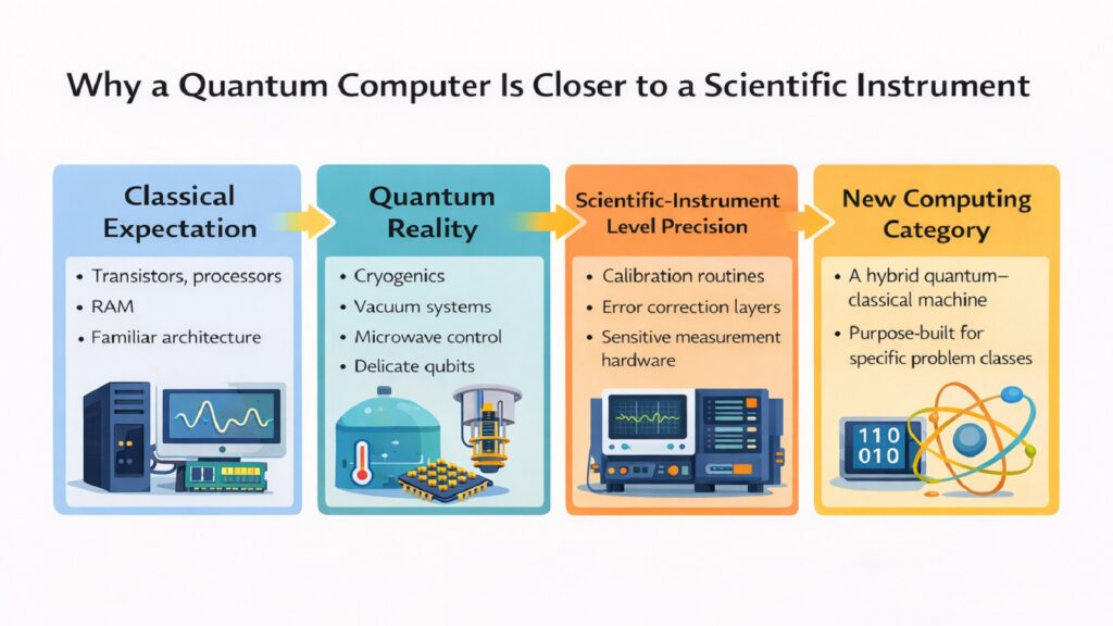
A Quantum Computer occupies a technological category between a scientific instrument and a computing machine. It requires trained operators, constant calibration, and environmental conditions matched only by physics laboratories. The next decade will determine whether engineering advances can reduce these requirements sufficiently for broader deployment. Regardless of that outcome, the Quantum Computer remains one of humanity’s most sophisticated attempts to harness fundamental physics for practical computation. The components described here represent not just engineering challenges overcome but a new understanding of how to manipulate reality at its smallest scales.
Quantum Computer Development Trajectory
| Aspect | Current Status |
|---|---|
| Qubit Count Trend | Doubling approximately every two years, currently reaching several hundred qubits |
| Error Rate Improvement | Gate fidelities improving from 99 percent to 99.9 percent over past decade |
| Coherence Time Progress | Increasing from microseconds to hundreds of microseconds through materials research |
| System Cost | Complete systems ranging from 10 million to over 30 million dollars |
| Operating Cost | Annual operating expenses of 500,000 to 2 million dollars including maintenance |
| Application Readiness | Drug discovery and materials science approaching practical utility thresholds |
| Scaling Challenge | Each additional qubit requires proportional infrastructure creating engineering limits |
| Timeline to Advantage | Quantum advantage for specific real-world problems expected within five years |
Read More Tech Articles
- Machine Learning in AI: 6 Powerful Ways AI Learns
- Quantum Computing: 6 Powerful Concepts Driving Innovation
- 8 Powerful Smart Devices To Brighten Your Life
- Canva Magic Media Review: 8 Reasons Why It is Unique
- 8 Big Ways Aged People Are Benefitting From Smartphones
- 8 Big Ways Female Entrepreneurs Are Benefiting From FinTechs
- 8 Best AI Image Generators That You Must Know About
- AI Images: 8 Simple Steps To Create Images Using AI